Vision Language Action Model Development & Validation
 by Kevin Cloutier, August 12, 2026
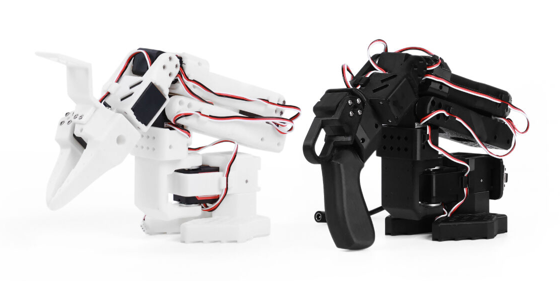
This research explores the use of Vision-Language-Action (VLA) models to control a physical robot and perform a real-world pick-and-place task. A VLA model is designed to connect three things: what the robot can see, what it has been told to do, and the actions it should take. In practical terms, the model receives visual observations from the robot's cameras, a language description of the task, and information about the robot's current state, then predicts a sequence of actions for the robot to execute. This is different from traditional robotic programming, where an engineer typically defines explicit coordinates, trajectories, rules, and conditions for every step of a task. A VLA instead learns a relationship between observations, instructions, and actions from examples. This makes the approach particularly interesting for tasks where the environment and object locations can vary and where explicitly programming every possible situation would be impractical.
Before you Begin
This research assumes you have already completed the SO-101 setup and configuration guide, including assembling and configuring the robot, connecting the required cameras, and verifying that the robot is operational with LeRobot. If you have not completed that setup, please follow the SO-101 guide first. This page focuses on the VLA research workflow and assumes the underlying robot environment is already working.
Resources
SmolVLA & LeRobot
At the center of this research is SmolVLA, a relatively compact VLA foundation model developed by Hugging Face. A foundation model provides a general starting point rather than being trained specifically for one robot or one task. The intention is that the model already contains useful learned representations and capabilities that can then be adapted to a particular application through fine-tuning. In this project, I am fine-tuning SmolVLA using demonstrations collected from a SO-101 robot performing a specific pick-and-place task. The objective is to investigate how effectively a pre-trained VLA can be adapted to a constrained physical task using task-specific data.
LeRobot provides much of the infrastructure connecting the model to the physical robot. Developed by Hugging Face, LeRobot provides tools for recording demonstrations, managing robotic datasets, training and evaluating policies, and communicating with supported robot hardware. It therefore acts as the practical framework around the VLA: the robot and cameras generate observations, LeRobot structures those observations into training data, SmolVLA is fine-tuned on that data, and the resulting policy can then be deployed back onto the robot to generate actions. This creates a complete development loop from data collection → training → inference → physical evaluation.
The purpose of this research is to examine that entire loop rather than simply demonstrate that a trained model can successfully move a cube. I am evaluating how the quality and configuration of the training data affect performance, how sensitive the resulting policy is to changes in the robot's starting position and environment, how inference latency affects real-time control, and whether a custom control system can reliably execute the actions produced by the model. I am also comparing LeRobot's built-in tools with my own control and evaluation software. This provides an important distinction between model failures and implementation failures: if the same model behaves differently when driven by two independent control systems, the problem may lie in the software pipeline rather than in the model itself. Ultimately, the goal is to understand not just whether SmolVLA can perform this task, but what is required to make a foundation-model-based robotic system reliable enough to move from an experimental demonstration toward a repeatable engineering system.
Research Roadmap
This page is Part 1 of the research and focuses on developing, training, and validating the VLA system. Part 2 will take the resulting model and custom inference software and investigate deployment across heterogeneous edge hardware.
The Approach
A simple web search will reveal countless articles focussed on creating a Hello World using the SO-101 robotic arms along with Hugging Face and the LeRobot framework. Most are fantastic and can accelerate one's understanding of Physical AI. But at the same time, many are trivial examples that overlook the complexities of what they are attempting to convey and gloss-over the edge-cases where all goes wrong. More often than not, there is little more than a few result videos showing perfect scenarios without addressing how one could overcome failures associated with this gargantuan effort. Here at Cloutier.engineer, my focus is bit deeper where I focus a level or two below the surface, meandering all the way down to the compute hardware and device execution (e.g. CPU, GPU, NPU, etc).
From Model to Metal
This is a good time to address cloud computing. Much of what you read on Cloutier.engineer can be replicated in the cloud, and for many applications, that is exactly the right approach. There are, however, some important exceptions. I regularly work with pre-release hardware, ranging from discrete GPUs to engineering samples, where access to the physical device is essential. More broadly, I deliberately acquire and run much of my experimental hardware locally.
Why? Because I want to understand the entire pipeline, not just the parts that are visible through a cloud API. Running locally gives me control over the hardware, software stack, drivers, runtimes, inference engines, and ultimately the device execution itself. It also forces me to understand what is actually happening beneath the abstraction layers rather than relying on a conveniently named service to handle those details somewhere behind the scenes. But don't be fooled, this also creates many headaches, roadblocks, and is 100% not for the faint of heart.
This hands-on approach is a significant part of what I am trying to explore here. The goal isn't simply to make something work, it is to understand why it works, where it fails, and what is happening at every layer along the way.
Similar to most other research here at Cloutier.engineer, I use Docker containers to ensure I don't pollute host machines while creating a reliable and repeatable environment. The Dockerfiles for this experiment fall into three categories that are aligned with the hardware described below: Data Acquisition, Training, and Inference.
This categorization is further divided into compute stacks such as NVIDIA DGX Spark-specific, Intel Up Xtreme machines, and more. This may seem like overkill, but this infrastructure allows me to easily revisit the experiment with additional environments (e.g. using an Intel ARC B70 instead of the DGX spark for training. Or utilizing a NVIDIA Jetson Orin Super Development Kit for inference instead of an Panther Lake-based system, etc.). In the end, I want to be able to quickly extend this research when the postal carrier delivers the new hardware du jour.
The containers are configured for specific versions of the LeRobot source code which is installed during the build. This is done to ensure I have 100% confidence that any issue which arises in the future is not an artifact of a new breaking-change that came down in an update. This is a great way to avoid those issues, but it is not without drawbacks. First, the checkout I selected did have a few minor issues that I discovered when "using the system in anger". I fixed these with patch files that you can evaluate by examining the DockerFile for specific comments. Additionally, as time goes on, the checked-out API slowly drifts away from the latest available version, thus resolving unknown issues by crowdsourcing becomes harder as the amount of people using this version declines. With that said, using this methodology is the best way to ensure my experiments are repeatable.
Also note that during the Docker image build process several environment variables are set so that LeRobot and Hugging Face behave a bit differently than the vanilla out of the box installations. Looking at the docker file, three of the variables are important to understand: HF_LEROBOT_HOME, HF_HOME, and HF_HUB_OFFLINE.
-
HF_LEROBOT_HOME: Defines the root directory LeRobot uses for datasets, model checkpoints, calibration data, and cached assets. By default this is a hidden directory called .cache in your users home directory (e.g. ~/.cache). Why on God's earth was it decided to default to hiding this directory? No idea, but thankfully this is easy to change by setting the HF_LEROBOT_HOME environment variable. You will see this has been set to /app/data.
-
HF_HOME: The Hugging Face Home directory, similar to HF_LEROBOT_HOME, this defaults into the ~/.cache directory. For similar reasons, I moved this to within the /app/data folder.
-
HF_HUB_OFFLINE: Last but not least, this flag forces the Hugging Face libraries to operate entirely offline. When set, model loading, dataset access, and cache lookups use only local files and never contact the Hugging Face Hub. There is an exception here, the `tokenizer_name` setting in the smolvla_base we download during build (I pre-download the policies I need, so there is no reason to communicate with the Hugging Face cloud post-build) is incorrectly hardcoded to force an online check, which of course fails when this flag is set. Take a look at the Dockerfile and you will see the patch created to fix this issue, which surely has been fixed in later versions of the software. So, in these environments, HF_HUB_OFFLINE is set to 1, stoping communications with the Hugging Face Hub.
As is the case with all examples here, the documentation on how to build the image and run the container is provided within each Dockerfile. If you are looking to follow along, download the Resource Kit and spin up the corresponding environment for whichever task you wish to reproduce (e.g. data acquisition, training, inference) or create your own setup targeting your hardware leveraging these files as a guide.
Data Acquisition Compute
When working on large scale imitation learning projects a team of people are often tasked with acquiring training data. You may have even seen videos online showcasing huge warehouse-like environments with technicians running robotic arms, recording data. This can also be a group of software engineers creating simulated data, or even a myriad of different combinations of humans, simulations, etc. The only certainty is that the data acquisition (or, when simulating, "data creation") will occur on dedicated machines.
In this research, my data acquisition rig is an AMD Ryzen Threadripper with 12 physical cores containing 2 threads each, resulting in 24 logical CPUs (threads). Details from lscpu below:
Architecture:             x86_64
  CPU op-mode(s):         32-bit, 64-bit
  Address sizes:          43 bits physical, 48 bits virtual
  Byte Order:             Little Endian
CPU(s):                   24
  On-line CPU(s) list:    0-23
Vendor ID:                AuthenticAMD
  Model name:             AMD Ryzen Threadripper PRO 3945WX 12-Cores
    CPU family:           23
    Model:                49
    Thread(s) per core:   2
    Core(s) per socket:   12
    Socket(s):            1
    Stepping:             0
    Frequency boost:      enabled
    CPU max MHz:          4000.0000
    CPU min MHz:          2200.0000
    BogoMIPS:             7985.75
Let's stop and think about what it is we are doing. For this research I have one Leader and One Follower arm. The Follower arm has an OpenCV camera mounted to its gripper and a RealSense d415 camera is mounted as a "World Camera" above the table, pointed at a slight downward angle so it can see the entire setup (including the Follower robot). When recording training data we are leading the follower robot (over USB); recording server motor states (over USB); recording video from the OpenCV wrist-mounted camera (over USB); and recording video from the RealSense world-context camera (yes, you get the idea, this is by USB too). That's a lot going on at the same time.
Now, my training rig is a beast. As noted above, it's an AMD Threadripper with 24 CPU cores, a ton of RAM, and a dedicated NVIDIA 5060 RTX TI with 16gb of VRAM. Awesome, right? Well, let's think about this a bit further. The graphics card excels during training and inference, but it's not used at all during data collection. Ok, but 24 cores and a ton of RAM still means we can fly to the moon with this machine, right? Well, yes, and no.
The LeRobot framework has a "million" configuration parameters and setting one incorrectly can cause what is known as “CPU starvation”. CPU starvation does not mean the computer's CPU is fully overloaded. Instead, it indicates that the real-time recording loop failed to complete a cycle within the required time budget (typically 33ms for a 30 Hz loop). Additionally, the recording loop is single-threaded, if any part of the pipeline blocks the thread (e.g. camera capture, image preprocessing, etc.), then Python's Global Interpreter Lock (GIL) loop misses its deadline. When this happens, LeRobot prints a “CPU starvation” warning even if many CPU cores are idle. This was the bane of my existence for longer than I will ever admit.
"But it's just a warning, why do I care?". In fact, "CPU starvation" is just a warning but it means your data acquisition is running below the standard 30 Hz, dropping frames and data along the way. In my case, when I started this effort I was often running at 6 Hz even on the Threadripper ("1.21 Gigawatts!!!"). Dropping that much data means a model trained on data recorded in this manner will behave in strange, unpredictable ways. In a pick-and-place scenario this results in tremendous jitter. Trust me, I know.
Training Compute
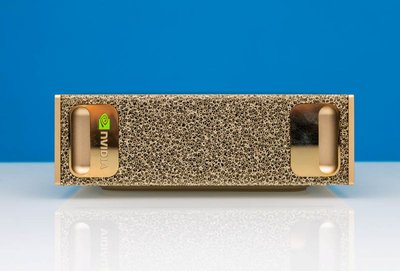
The NVIDIA DGX Spark serves as the sole training environment for this research. It provides the dedicated compute resources used to train and fine-tune machine learning models, including the LeRobot/SmolVLA policies I am experimenting with here. Once training datasets are acquired, they are preprocessed and then stored on a local NAS. This means the data acquisition workflow is simple, acquire the data, pre-process (combine episodic training), and save it to the NAS. That's it.
When training is about to commence, I transfer the data over the high-speed internal lab network to the DGX spark. By consolidating training here on the Spark, this environment can remain consistent and reproducible across multiple experiments, while data acquisition and inference can remain isolated from the resource-intensive training workload as it is in most professional environments (e.g. engineers are not running all steps of the imitation learning pipeline on one machine). Additionally, this setup means I can be training a model on the Spark, running data acquisition on the Threadripper, and running inference on multiple edge devices (described below) at the same time.
Inference Compute
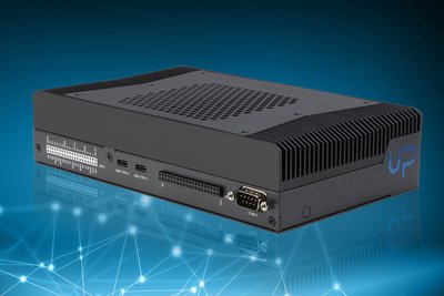
I am currently using the AAEON UP Xtreme PTL Edge, evaluating Intel's Core Ultra Series 3 platform that consists of a CPU, iGPU, and an NPU accelerator. This box is in fact the real impetus for this experiment. I am attempting to evaluate the SoC for this type of workload at the edge. The platform is rated for up to 180 TOPS of combined AI performance, I want to see how it performs in the real world. Similar to the other environments listed above, this box is intentionally isolated from data acquisition and model training and is used exclusively to deploy and execute trained models. This allows inference performance, latency, resource utilization, real-world robotic workloads, and everything in between to be evaluated in its own silo.
Camera Extrinsics
Camera extrinsics describe where a camera is located in the physical world and how it is oriented relative to a fixed reference frame. In robotics, this reference frame is typically the robot's workspace or a calibration board mounted in a known, stable position. Without accurate extrinsics, any 2D detection such as AprilTags, objects, barcodes, cannot be reliably converted into 3D world coordinates. The robot may “see” an object, but it has no trustworthy way to determine where that object is physically located.
At the start of all training sessions, I place a precisely sized AprilTag (56 mm x 56 mm black square) at a known location mounted to the robot arm. Doing so allows me to solve for the camera's full 6-DoF pose providing both the rotation and translation of the camera relative to the AprilTag and thus the robot. Once solved, I store this transform as static metadata and use it to recalibrate the experiment setup later.
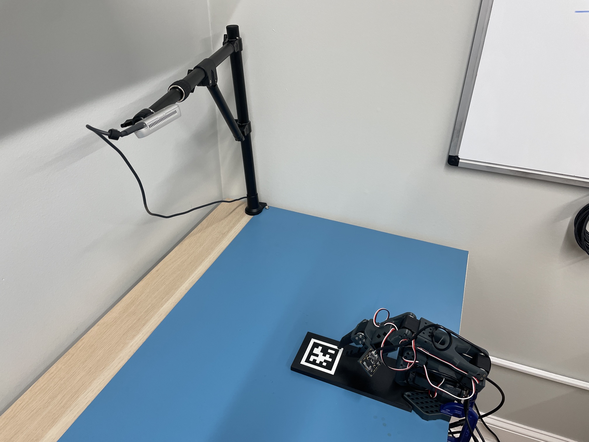
The location of the cameras matter because the Vision-Language-Action model learns from the world as the camera saw it during training. At inference time, the model assumes the camera is still in that same pose. If the camera moves, even slightly, the model's predicted actions will be spatially misaligned. And yes, this absolutely happens in real deployments. If you've ever torn down your demo, shipped it across the globe, and rebuilt it on a different table (hello, Hannover Messe!!!), the world camera will not be in the same physical location.
Fortunately, the fix can be simple: place the camera in a roughly similar position, run the same vision extrinsics routine that was run during training. Determine if the camera is mounted within an acceptable range of deviation, and if not, keep adjusting it until it's correct.
This concept can be taken much further by using the current extrinsics data together with the saved training metadata to compute a transformation to align inference-time action chunks with training-time coordinates. But that's gold-plating I don't need at the moment, and a great issue for a full research article here at Cloutier.engineer.
What about the Wrist Camera?
The World Camera is an external sensor mounted to the table or demo environment. Its position can change from setup to setup, event to event, or even after someone bumps the rig with an insanely large backpack while you are getting a cup of coffee (again, I am looking at you Hannover Messe!!!). Because its pose is not guaranteed, we must calibrate it each time to recover its true location within the world frame.
The Wrist Camera, on the other hand, is rigidly mounted to the robot's end-effector. Its pose relative to the robot is fixed, known, and repeatable. The robot's kinematics already define exactly where the gripper camera is at any moment. This means the gripper camera's extrinsics are effectively “built in” to the robot model and do not need to be recalibrated unless the physical hardware changes.
Vision Calibration
My custom vision_calibration library (found in the Resources bundle) provides a complete, automated pipeline for computing the camera extrinsics of the World Camera. The library handles all steps of the calibration process: capturing an image from the RealSense world camera, detecting AprilTags on the board, building 3D-2D correspondences, and solving the Perspective-n-Point (PnP) problem using the camera's intrinsic parameters and distortion coefficients. The result is a single 4x4 homogeneous transform, T_world_cam, which expresses the camera's pose in the world frame relative to the AprilTag.
Like most of Cloutier.engineer, vision_calibration is a work in progress, more akin to a beta than a production grade system. But it works, and I will be adding additional features as I incorporate it into the larger breadth of this work. To run a test example, grab the code, a camera, an AprilTag, and execute the below code. The --tag-id argument is informing the system which tag to find. For example, if your camera can see multiple tags, vision_calibration needs to know which you are interested in basing your extrinsics. In this example, I am using an AprilTag that represents the number 1. If you don't have a tag handy, you can create your own at https://chev.me/arucogen/. Note: vision_calibration currently only supports the 36h11 format.
python3 tests/AprilTags.py --tag-id 1 --output-path .
The program automatically saves a serialized numpy array, T_world_cam, at the location provided with the output-path argument. T_world_cam contains two components: a rotation matrix and a translation vector.
-
Rotation Matrix: Rows 1-3, columns 1-3, these nine values define the camera's orientation relative to the board. Numbers close to 1 on the diagonal indicate the camera is facing the board with only a slight tilt. Each row represents one of the camera's local axes expressed in world coordinates.
-
Translation Vector: Rows 1-3, column 4, these three values define the camera's position in world space in meters:
- X = 0.0355 m - The camera is ~3.5 cm to the right of the tag center.
- Y = -0.0122 m - The camera is ~1.2 cm below the tag center in world Y.
- Z = 0.4676 m - The camera's optical center is ~46.8 cm above the board. This Z value is the most important: it tells you the camera's actual height above the workspace.
-
Homogeneous Transform Footer: Row 4, the final row [0 0 0 1] makes the matrix compatible with standard robotics math, allowing it to be used for transforming points between coordinate frames.
In summary, this matrix fully describes where the World Camera is currently located and how it is oriented relative to the calibration board. This is key for being able to reproduce camera extrinsics seen during training at inference time. I recommend saving this output directly alongside of your training data.
AprilTag Example Code
---------------------
Intrinsics of Camera are:
	Width: 640
	Height: 480
	fx: 605.1539306640625
	fy: 603.8364868164062
	ppx: 320.7110290527344
	ppy: 232.15142822265625
	Distortion model: distortion.inverse_brown_conrady
	Distortion coeffs: [0.0, 0.0, 0.0, 0.0, 0.0]
Searching for all tags
Detected 1 tags: [1]
Get camera extrinsics for ApriTag ID == 1
T_world_cam (camera pose in world frame):
[[ 0.9992688  -0.01817334  0.0336399   0.03553643]
 [ 0.02045992  0.99741197 -0.06892582 -0.01223235]
 [-0.03230023  0.06956369  0.99705446  0.46756023]
 [ 0.          0.          0.          1.        ]]
Data Collection Strategy
The official SmolVLA guidance recommends a baseline of 50 episodes for real-world tasks. This is a minimum recommendation, much more data is required for more complex tasks. But for a simple pick-and-place task it is often enough. The objective is straightforward: pick the object from a different starting position in each episode and place it in the correct destination.
What Is an Episode?
An episode is one complete execution of a task, beginning from a defined starting state and ending when the task is completed. For this research, one episode consists of the bench containing a 1x1 inch red cube in a particular location, the robot moves to the cube, grasps it, transports it to a white dish, releases it, and then returns to the start. That is actually more complex than it may sound.
Each episode therefore represents one example of the robot performing the complete pick-and-place task. While the task itself remains the same from episode to episode, the cube's starting position varies. This variation provides the model with multiple examples of the same behavior while preventing it from simply memorizing a single trajectory.
For this initial experiment, the cube is placed on a lab bench covered with a uniform blue ESD material. This intentionally controlled environment reduces unnecessary variability in the visual background while keeping the object and its destination well defined. By limiting the number of variables the model must account for, we can focus on whether it can reliably learn the fundamental pick-and-place behavior.
The figure below illustrates the task.
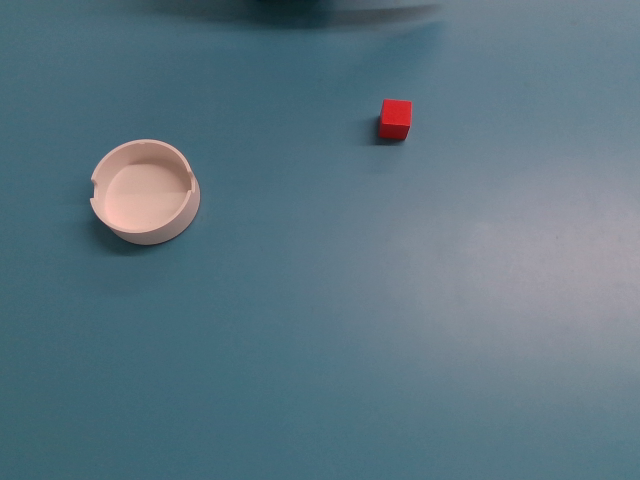
Using the above scenario, we are teaching the robot (creating a policy) that the “pick” isn't a single coordinate, but any location within a particular area. After “picking”, we place the item into the white dish. In reality, we could pick and place from and to anywhere, but this strategy will keep things simple. During these training sessions we will only have one item to pick on the bench at a time. Multiple items are possible, but that would increase the complexity of this experiment and likelihood of failure.
Once the cube has been placed, I move the robot back to a "home" position. This ensures that the next pick starts form the same position and the robot is not blocking the view of the world camera for the next recording. Let's look at a few episodes of a training video from two vantage points, the "world" and "wrist" cameras:
Let's review a few LeRobot settings I found useful in my setup to vanquish the "CPU starvation" warning. Remember, your model is only as good as the data you collect:
-
display_data: Enables live visualization of incoming camera frames and robot observations during recording. This is useful for seeing the data in realtime via Rerun on your host. But, I find the overhead is immense. Be sure to set this to FALSE
-
dataset.streaming_encoding: When enabled, video frames are encoded and written to disk in a streaming fashion. This can make training sessions quicker and reduce memory usage but it has the result of drastically increasing CPU load. Setting this to FALSE will add ~five seconds of post-processing time to each episode, but that can be mitigated by setting the dataset.reset_time_s to 0. In the past I used a 5 second reset to allow me time to physically move the cube back to the start and ready myself for the the next episode. Setting this to 0, along with dataset.streaming_encoding=false, and it's basically the same length of time.
-
dataset.encoder_threads: Sets the number of parallel CPU threads used for video encoding. I find using 4 is the sweet spot for my rig, your mileage may vary.
-
dataset.num_image_writer_processes: Sets the number of separate processes responsible for writing image files to disk, improving throughput on fast storage but adding system overhead. I found 2 works best with the two camera setup here.
-
dataset.vcodec: This is a big one... vcodec selects the video codec used to encode camera streams (e.g., h264), which determines compression efficiency, file size, and what device the encoding happens on. For example, setting this to h264_nvenc requires the encoding to be done on the GPU. Good, right? Wrong... That means each image needs to be moved from the CPU to the GPU for processing. Since we are trying to process 30FPS, that's a lot of data moving to the dedicated GPU. I found setting this to h264 drastically reduces CPU pressure by keeping the encoding on the CPU (I know, counterintuitive).
In the end, a command like the below is what I needed to acquire my training datasets without starving the CPU and ensuring that each and every piece of data was saved. Note, pay close attention to the log streaming to the terminal. Every single warning is important, try to eradicate them all before training a model.
In the command (lerobot-record) you will see the use of environment variables $PROMPT and $CURRENT_JOB. This is done to improve the usability of these commands as the same data is used in multiple commands from training to inference. Using ENV variables is a simple way to reduce the chance of error when moving between commands. For example, getting the prompt wrong at one stage can impact the entire training cycle.
-
PROMPT: The prompt is the text I feed into the model describing the action we want to take. For example: "Pick the red cube and place it into the white dish". Even though we are manually manipulating the robot, we need the model to learn that the provided prompt is used to request this action at inference time.
-
CURRENT_JOB: This represents the name of the job, for example: "pick-and-place-simple". Each data collection session will output data using this name and a timestamp. That latter part, the timestamp, allows one to record the same data over and over again without having file / folder name collisions.
########################################################
# Note, I use PYTHONUNBUFFERED=1 here as it
# tells Python not to buffer its output. In other words,
# it forces Python to write everything to stdout and
# stderr immediately, instead of waiting and flushing
# in chunks. This can help during debugging.
########################################################

PYTHONUNBUFFERED=1 lerobot-record \
    --display_ip=127.0.0.1 \
    --display_data=false \
    --play_sounds=true \
    --dataset.single_task="$PROMPT" \
    --dataset.repo_id="local/${CURRENT_JOB}_$(date +%Y%m%d_%H%M%S)" \
    --dataset.num_episodes=5 \
    --dataset.streaming_encoding=false \
    --dataset.encoder_threads=4 \
    --dataset.num_image_writer_processes=2 \
    --dataset.push_to_hub=false \
    --dataset.vcodec=h264 \
    --dataset.reset_time_s=0 \
    --teleop.type=so101_leader \
    --teleop.port=/dev/so101-leader-1 \
    --teleop.id=so101-leader-1 \
    --robot.type=so101_follower \
    --robot.port=/dev/so101-follower-1 \
    --robot.id=so101-follower-1 \
    --robot.cameras='{
        "camera1": {
                "type": "intelrealsense",
                "serial_number_or_name": "220222063537",
                "width": 640,
                "height": 480,
                "fps": 30,
                "warmup_s": 2
        },
        "camera2": {
                "type": "opencv",
                "index_or_path": "/dev/so101-follower-1-opencv_gripper_cam",
                "width": 640,
                "height": 480,
                "fps": 30,
                "warmup_s": 2
        }
    }'
Using the videos and command above, collect data as described in the table below. Each session should be its own dataset. If you make a mistake, the easiest thing to do is delete the entire dataset and start over. Yes you can trim a dataset with the LeRobot CLI, but most often it's easier to just start anew.
Goal |
Description |
Episodes |
|---|---|---|
Establish a clean baseline. |
|
5 |
Small X Variation: Test sensitivity to distance from the robot. |
Move the cube slightly:
|
5 |
Larger X Variation: Expand the distance variation. |
Use five progressively different X positions:
Don't push the cube into an obviously unreachable or problematic location. |
5 |
Small Y Variation: Test lateral sensitivity. |
Keep X approximately constant and move the cube left/right across the workspace:
|
5 |
Larger Y Variation: Push the lateral workspace variation further. |
Again, keep X fixed but move across the Y axis:
|
5 |
X + Y Grid: Test combinations rather than changing one dimension at a time. |
Use five distinct locations:
This starts testing whether the model struggles with particular regions of the workspace rather than simply X or Y independently. |
5 |
Workspace Extremes: Find the boundaries of reliable operation. |
Use five locations near the practical limits of the trained workspace:
Don't intentionally create impossible grasps, the goal is to find the edge of the model's learned workspace, not the mechanical limits of the robot. |
5 |
Randomized Workspace: Introduce realistic variation. |
Choose 15 locations without following an obvious pattern. They should all be within the reasonable workspace of the training data, but not necessarily positions you've used before. |
15 |
Dataset Merging
As was seen earlier, the lerobot-record functionality allows you to select how many episodes to record, but 50 (the number suggested by SmolVLA, normally I record much more, minimum of 75) is a lot to do in one sitting. I always divide this into smaller sessions, for example, 10 sessions of 5 episodes each. As long as you keep the environment the same (same cameras, same camera locations, same resolution, etc.), you can combine datasets taken at different times (even different days) into one training set with the LeRobot CLI. This allows you to continue to add datasets and fine-tune your models over and over.
I combine my data like so, again taking advantage of the environment variables set earlier:
# Create a comma-separated list of sessions.
#
# BE CAREFUL TO ONLY INCLUDE DATA WITH THE SAME PROMPT, ENVIRONMENT, ETC.
#
DATASETS=$(ls $HF_LEROBOT_HOME/local/ | grep "^$CURRENT_JOB" | sed "s|^|'local/|" | sed "s|$|'|" | paste -sd "," -)

#
# Merge the training into one data set
#
lerobot-edit-dataset \
   --new_repo_id "local/$CURRENT_JOB-merged" \
   --operation.type merge \
   --operation.repo_ids "[$DATASETS]"
The output will look similar to the below with a new dataset saved at the end. Note the above command appends "_merged" to the CURRENT_JOB variable to denote this is all of the datasets combined.
INFO 2026-07-29 21:00:46 _dataset.py:393 Loading 10 datasets to merge
INFO 2026-07-29 21:00:46 eo_utils.py:108 Using video codec: libsvtav1
INFO 2026-07-29 21:00:47 eo_utils.py:108 Using video codec: libsvtav1
INFO 2026-07-29 21:00:47 eo_utils.py:108 Using video codec: libsvtav1
INFO 2026-07-29 21:00:47 eo_utils.py:108 Using video codec: libsvtav1
INFO 2026-07-29 21:00:47 eo_utils.py:108 Using video codec: libsvtav1
INFO 2026-07-29 21:00:47 eo_utils.py:108 Using video codec: libsvtav1
INFO 2026-07-29 21:00:47 eo_utils.py:108 Using video codec: libsvtav1
INFO 2026-07-29 21:00:47 eo_utils.py:108 Using video codec: libsvtav1
INFO 2026-07-29 21:00:48 eo_utils.py:108 Using video codec: libsvtav1
INFO 2026-07-29 21:00:48 eo_utils.py:108 Using video codec: libsvtav1
INFO 2026-07-29 21:00:48 _dataset.py:398 Merging datasets into local/pick-and-place-simple-merged
INFO 2026-07-29 21:00:48 ggregate.py:261 Start aggregate_datasets
Validate all meta data: 100%|██████████████████████████████████████████████████████████████████████████████████████████████████████████████████████████████████████████████████████████████████| 10/10 [00:00<00:00, 133152.51it/s]
INFO 2026-07-29 21:00:49 ggregate.py:292 Find all tasks
Copy data and videos: 100%|████████████████████████████████████████████████████████████████████████████████████████████████████████████████████████████████████████████████████████████████████████| 10/10 [00:03<00:00,  2.77it/s]
INFO 2026-07-29 21:00:52 ggregate.py:639 write tasks
INFO 2026-07-29 21:00:52 ggregate.py:642 write info
INFO 2026-07-29 21:00:52 ggregate.py:653 write stats
INFO 2026-07-29 21:00:52 ggregate.py:320 Aggregation complete.
INFO 2026-07-29 21:00:52 eo_utils.py:108 Using video codec: libsvtav1
INFO 2026-07-29 21:00:52 _dataset.py:405 Merged dataset saved to /app/data/local/pick-and-place-simple-merged
INFO 2026-07-29 21:00:52 _dataset.py:406 Episodes: 50, Frames: 21798
Dataset Evaluation
This could be the most important aspect of imitation learning pipelines that is often overlooked in online tutorials. Recording data is difficult, time consuming, and error prone. Unfortunately, those errors often go unnoticed during data acquisition and can seep into your training sessions sometimes destroying your models effectiveness. One bad episode of 50 can ruin the entire model. Therefore it is imperative you evaluate your data before using it. I use two main methods, the LeRobot-Doctor and custom visualization scripts.
LeRobot Doctor
lerobot-doctor is a diagnostic tool designed to help identify common issues in LeRobot environments, datasets, hardware, and training configurations. It provides a structured way to inspect a LeRobot installation and surface potential problems that can negatively affect data collection, training, or policy inference. And of course, it's part of the Docker container supplied in this research.
Imitation Learning projects, and specifically anything with SmolVLA, has proven debugging can be the most difficult part. This is because poor results can come from so many different sources: incorrect configuration, dataset problems, hardware or camera issues, software dependencies, or even training settings. LeRobot-Doctor helps narrow down these possibilities by checking the environment and configuration, giving us a starting point for troubleshooting before making changes to the training pipeline.
Let's look at the output of this program on the dataset I used for this research. You can replicate this on your own dataset with the following command:
lerobot-doctor /path/to/your/dataset/
And the output:
lerobot-doctor v0.2.0 -- Dataset Quality Report
Dataset: data/local/simple-merged (v3.0)
Episodes: 75 | Frames: 25,769 | FPS: 30

[PASS] Metadata & Format Compliance

[PASS] Temporal Consistency

[WARN] Action Quality
  - action: 10% of episode 0 is consecutive identical actions (frozen)
  - action: 12% of episode 1 is consecutive identical actions (frozen)
  - action: 12% of episode 2 is consecutive identical actions (frozen)
  - action: 12% of episode 3 is consecutive identical actions (frozen)
  - action: 13% of episode 4 is consecutive identical actions (frozen)
  - action: ...and 59 more episodes with frozen actions

[PASS] Video Integrity

[PASS] Data Distribution

[PASS] Episode Health

[PASS] Feature Consistency

[PASS] Training Readiness

[WARN] Anomaly Detection
  - observation.state[5]: stuck/static in 65/75 episodes (>80% unchanged each) -- possible stuck actuator or unused DOF

[PASS] Portability

[WARN] Per-Episode Summary
  - 64/75 episode(s) flagged
  - Episode 0: 10% of action frozen (consecutive identical)
  - Episode 1: 12% of action frozen (consecutive identical)
  - Episode 2: 12% of action frozen (consecutive identical)
  - Episode 3: 12% of action frozen (consecutive identical)
  - Episode 4: 13% of action frozen (consecutive identical)
  - Episode 5: 6% of action frozen (consecutive identical)
  - Episode 6: 7% of action frozen (consecutive identical)
  - Episode 7: 7% of action frozen (consecutive identical)
  - Episode 8: 10% of action frozen (consecutive identical)
  - Episode 9: 5% of action frozen (consecutive identical)
  - Episode 11: 11% of action frozen (consecutive identical)
  - Episode 12: 9% of action frozen (consecutive identical)
  - Episode 13: 13% of action frozen (consecutive identical)
  - Episode 14: 8% of action frozen (consecutive identical)
  - Episode 15: 12% of action frozen (consecutive identical)
  - Episode 16: 5% of action frozen (consecutive identical)
  - Episode 17: 7% of action frozen (consecutive identical)
  - Episode 18: 10% of action frozen (consecutive identical)
  - Episode 20: 5% of action frozen (consecutive identical)
  - Episode 22: 7% of action frozen (consecutive identical)
  - ...and 44 more flagged episodes

Summary: 8 PASS | 3 WARN
Interpreting this data is straightforward, though you have to look at this within the context of the experiment. What we see above is 8 PASS and 3 WARN. This looks mostly healthy, with two things worth investigating:
-
Frozen actions: 64/75 episodes have some frozen action, typically 5-13% of the episode. That's significant enough to investigate, but not necessarily fatal.
-
observation.state[5]: This is the bigger red flag. Joint 5 is static in 65/75 episodes, which strongly suggests that the DoF may not actually be changing or recording correctly.
Everything else passes, including temporal consistency, video, distribution, feature consistency, and training readiness. So, what is going on with the warnings? Well, this dataset is composed of only pick-and-place actions. observation.state[5]:, that's the gripper DoF. The report says it is static in 86% (65/75) of the episodes. Well, that's bad, right? Not necessarily, look closer. The comment also explains that the state of the gripper is ">80% unchanged" throughout the length of the episode. This does not say emphatically that the joint is not moving, we can only infer it is not moving much, which in this case, is 100% accurate. The gripper only opens when it approaches the cube, then closes, then reopens/closes to drop the cube. It seems that this action would in fact be less than 20% of the overall time. Let's investigate further.
Static Joint
We can create a simple Python script that extracts the data from test data, specifically the gripper joint, and plot it as seen in the below code snippet.
from lerobot.datasets.lerobot_dataset import LeRobotDataset
import matplotlib.pyplot as plt
import numpy as np

dataset = LeRobotDataset("/app/data/local/simple-merged")

episode = 0
data = dataset.hf_dataset.filter(lambda x: x["episode_index"] == episode)

states = np.array(data["observation.state"])
gripper = states[:, 5]

plt.plot(gripper)
plt.xlabel("Timestep")
plt.ylabel("Gripper position")
plt.title(f"Episode {episode} - Gripper")

plt.savefig("/app/logs/gripper_episode_0.png")
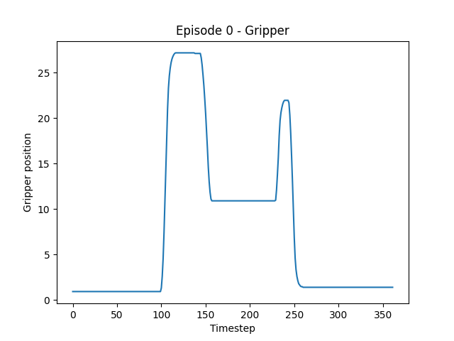
The gripper data is showing what I suspected, it starts closed, opens around timestep 100, stays open for about 50 steps, partially closes representing gripping the cube, then reopens around 235 showing the drop and subsequent closure / reset action. So the gripper is definitely functioning and changing state. It just spends a lot of the episode stationary, which explains the validation warning.
All Joints
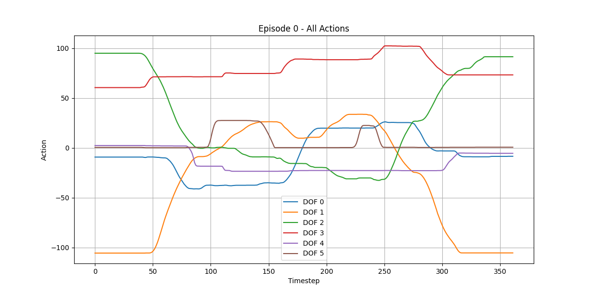
Now lets turn our eye to the other warnings, the n% of action frozen items. Following along with the above we can create a script that plots each degree of freedom on a single plot (including the original gripper joint seen above).
from lerobot.datasets.lerobot_dataset import LeRobotDataset
import matplotlib.pyplot as plt
import numpy as np

dataset = LeRobotDataset("/app/data/local/simple-merged")

episode = 0
data = dataset.hf_dataset.filter(lambda x: x["episode_index"] == episode)

actions = np.array(data["action"])

plt.figure(figsize=(12, 6))

for i in range(6):
    plt.plot(actions[:, i], label=f"DOF {i}")

plt.xlabel("Timestep")
plt.ylabel("Action")
plt.title(f"Episode {episode} - All Actions")
plt.legend()
plt.grid(True)

plt.savefig(f"/app/logs/actions_episode_{episode}.png")
plt.close()
The resulting plot is seen below, and it looks pretty healthy to me. The important observation is that the "frozen" periods are mostly intentional plateaus, not a dead control signal. Several joints hold position for long stretches while other joints move. DoF 3, for example, has long flat sections but clearly changes when needed. DoF 5 (gripper) has distinct open/close events as seen earlier, and there are no obvious periods where all 6 actions suddenly freeze simultaneously.
So the validator's 5-13% frozen-action warning looks to be expected for this task rather than evidence of bad data.
Frame Drops / Gaps
An important data point that is not addressed by the LeRobot-Doctor is dropped frames. If we are missing frames from our video then the model won't have the data it needs to create smooth actions. This can occur for many reasons, but in my experience I see this most often when the CPU is starved during data acquisition. A simple Python script can check for frames being dropped:
from lerobot.datasets.lerobot_dataset import LeRobotDataset
import numpy as np

DATASET_PATH = "/app/data/local/simple-merged"

EXPECTED_DT = 1 / 30
TOLERANCE = 0.010  # 10 ms

dataset = LeRobotDataset(DATASET_PATH)

episodes = np.array(dataset.hf_dataset["episode_index"])
timestamps = np.array(dataset.hf_dataset["timestamp"])

print("\nFrame Gap Check")
print("----------------")

total_gaps = 0
bad_episodes = 0

for episode in np.unique(episodes):
    mask = episodes == episode
    ts = timestamps[mask]

    if len(ts) < 2:
        continue

    dt = np.diff(ts)

    # Anything significantly larger than the expected frame interval
    gaps = np.where(dt > EXPECTED_DT + TOLERANCE)[0]

    if len(gaps) > 0:
        bad_episodes += 1
        total_gaps += len(gaps)

        print(f"\nEpisode {episode}: {len(gaps)} gap(s)")

        for i in gaps:
            print(
                f"  frame {i} -> {i+1}: "
                f"{dt[i]:.4f}s "
                f"(expected ~{EXPECTED_DT:.4f}s)"
            )

print("\n----------------")
print(f"Episodes with gaps: {bad_episodes}")
print(f"Total frame gaps:   {total_gaps}")
And the output shows no frame drops.
Frame Gap Check
----------------

----------------
Episodes with gaps: 0
Total frame gaps:   0
Length of Episodes
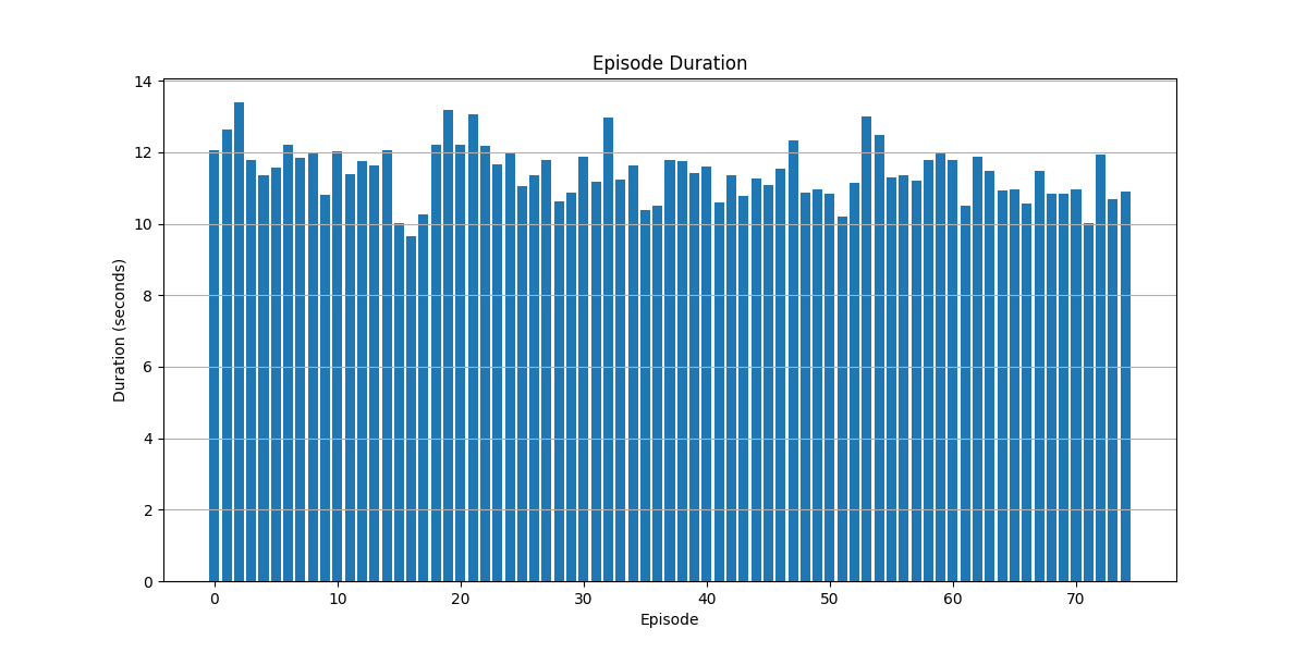
Finally we turn our attention to the length of episodes. What I am looking for here is similar length for each episode.
from lerobot.datasets.lerobot_dataset import LeRobotDataset
import matplotlib.pyplot as plt
import numpy as np

DATASET_PATH = "/app/data/local/simple-merged"
OUTPUT_PATH = "/app/logs/episode_durations.png"

FPS = 30

dataset = LeRobotDataset(DATASET_PATH)

episode_indices = np.array(dataset.hf_dataset["episode_index"])

durations = []

for episode in np.unique(episode_indices):
    frame_count = np.sum(episode_indices == episode)
    duration = frame_count / FPS
    durations.append(duration)

durations = np.array(durations)

print("\nEpisode Duration")
print("----------------")
print(f"Episodes: {len(durations)}")
print(f"Min:      {durations.min():.2f} s")
print(f"Median:   {np.median(durations):.2f} s")
print(f"Mean:     {durations.mean():.2f} s")
print(f"Max:      {durations.max():.2f} s")

# Plot
plt.figure(figsize=(12, 6))
plt.bar(np.arange(len(durations)), durations)

plt.xlabel("Episode")
plt.ylabel("Duration (seconds)")
plt.title("Episode Duration")
plt.grid(axis="y")

plt.savefig(OUTPUT_PATH)
plt.close()

print(f"\nSaved: {OUTPUT_PATH}")
As can be seen in the resulting plot, there is a good similarity in episode duration and it seems to be hitting that sweet-spot of 8-15 seconds as defined by SmolVLA documentation.
Evaluation Results
The dataset passes both LeRobot-Doctor and my additional custom validation plots. The results indicate that the data is statistically consistent, with no obvious problems such as stalled joints, unexpected motion, or significant frame loss. This gives me confidence that the dataset is suitable for training.
But what happens if these checks do reveal a problem? What if joints are actually stalling, frames are being dropped, or individual episodes contain corrupted or otherwise problematic data? In that situation, the safest approach is to first re-record the dataset and run the validation process again. Although data acquisition is time-consuming and is not necessarily the root cause of every problem, collecting a fresh dataset immediately eliminates the possibility that the original recording process or operator introduced the problem. If the same issue appears in the new dataset, we can then investigate the recording environment and software more systematically.
More commonly, the problem may be isolated to a relatively small number of episodes. In that case, the next step is to inspect the individual episodes, identify and remove those responsible for the anomalies, and retain only the highest-quality data. New recordings can then be appended to the cleaned dataset using the merge process described above. The important point is that dataset validation should not be treated as a formality. The quality of the data directly determines what the model has an opportunity to learn, and in my experience, this is one of the most important factors influencing the eventual success of the model.
Policy Creation (a.k.a. Training)
Now that the training data has been collected, validated, and merged, we can train the model. For this initial research, training was performed on the DGX Spark described above. You do not necessarily need this exact server-grade system; other GPUs can be used as long as they provide enough VRAM to hold the model and its associated training workload. If the available GPU memory is insufficient, training will fail or require a different configuration.
In the future, I plan to repeat this training process on an Intel Arc B70 and compare the results. I will update this documentation with those findings when that testing is complete.
Training time depends heavily on the number of steps and the hardware being used. As a rough reference, 20,000 steps can take several hours, while a larger 150,000-step run can take 12 hours or more. For this initial experiment, I recommend starting with 20,000 steps. This gives us a reasonable first model to validate before investing significantly more compute time in a longer training run. If the resulting model performs well, we can return later and train for additional steps to determine whether the extra training improves performance.
The training process continues to use the CURRENT_JOB and PROMPT environment variables established during data acquisition. Make sure these are still set correctly before starting. We will also introduce two additional variables:
-
POLICY_PATH: Specifies the filesystem path to the trained policy checkpoint that will be loaded for timezone_transitions_get. This basically tells the training script (lerobot-train) to load an existing baseline model instead of starting from scratch.
-
VLM_MODEL_NAME: While policy.path sets the container path for your entire robot policy, policy.vlm_model_name explicitly selects the underlying multi-modal AI model responsible for processing camera visual inputs and language instructions. It tells the LeRobot pipeline which specific pre-trained weights to pull down for the visual/language encoder
Let's set these variables so they can be used in the lerobot-train command.
# Set the environment variables
export POLICY_PATH="/app/data/huggingface/hub/models--lerobot--smolvla_base/snapshots/c83c3163b8ca9b7e67c509fffd9121e66cb96205"
export VLM_MODEL_NAME="/app/data/huggingface/hub/models--HuggingFaceTB--SmolVLM2-500M-Video-Instruct/snapshots/7b375e1b73b11138ff12fe22c8f2822d8fe03467"
Using the below command we can start the training process. Once completed, our model will have been saved into the output directory. Go take a look. You will find a checkpoints directory, which contains all of the checkpoints and a last directory that is a simlink to the last checkpoint. Inside of each checkpoint there will be directories for the information of the pre-trained model and training state.
#
# Let's move this train, choo-choo!
#
lerobot-train \
    --job_name="$CURRENT_JOB" \
    --dataset.repo_id="local/${CURRENT_JOB}-merged" \
    --steps=20000 \
    --save_freq=5000 \
    --wandb.enable=false \
    --policy.path="$POLICY_PATH" \
    --policy.vlm_model_name="$VLM_MODEL_NAME" \
    --policy.device=cuda \
    --policy.push_to_hub=false \
    --policy.empty_cameras=1 \
    --output_dir="$HF_LEROBOT_HOME/../models/${CURRENT_JOB}" \
    2>&1 | tee "$HF_LEROBOT_HOME/../models/${CURRENT_JOB}_training.log"
Training Results
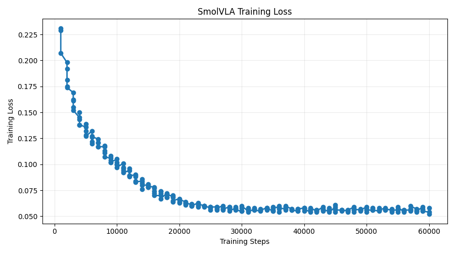
The training run provides our first quantitative look at how the model learned from the dataset. The graph above shows the SmolVLA training loss over 60,000 training steps. The loss falls rapidly during the early stages of training, dropping from approximately 0.20 at the beginning to around 0.10 by 10,000 steps. It continues to decrease more gradually before settling into a relatively stable range around 0.055–0.060 for much of the later training. The final recorded training loss was approximately 0.052.
This indicates that the optimization process is converging, but a decreasing training loss does not mean that the robot will necessarily perform the task successfully. The loss tells us how well the model is fitting the training objective, it does not tell us whether the resulting policy generalizes to the physical robot, different object positions, or real-world variations that were not present in the training data. To answer those questions, we need to take the next step and evaluate the trained policy against the actual robot.
Physical Validation
It is extremely important that we eliminate variables that can impact our outcomes during validation. This is true of actual usage in the field as well, but during evaluation we are attempting to determine why a model fails, not succeeds. We do this systematically and a good place to start is by running 10 inference sessions and taking notes, like seen in the below table from my initial run of SmolVLA data (the same data used to generate the plots shown earlier). The 10 first set of data points comes from using the built-in leRobot-record command. This command can be used to run inference when passed a policy path. I believe it is called record because it does in fact record the complete episode so you can evaluate it later.
The second ten data points come from the program I wrote to demonstrate this pick-and-place solution. Though the leRobot-record function is a great quick-and-dirty demo, it is not something one would use in the field. Rather, we would use a custom program that includes proper logging, threading, integrations to larger control systems, WMS, MES, etc. Can you guess the reason I don't only use this custom program? Correct. A Custom program is nearly by definition full of custom bugs not yet found. To ensure issues with model inference are not inserted by poor programming choices, I use both the custom program and the leRobot-record command. We should see similar output, and if we don't, that is cause for concern and further evaluation.
First let's look at the leRobot-record command. One of the key the key parameters is the --policy.n_action_steps (e.g., to 30). This is critical. Setting this to the maximum of 50 means that the policy will predict all 50 actions and all 50 will be played. If we set it to 1, the policy would predict only 1 action. Since each inference takes ~250ms, we need ensure we balance the amount of times we are running inference to reduce lag, etc. while also ensuring we are not consuming hallucinations that are likely at the backend of the max 50 actions. So, I usually use between 20 and 30, here I selected 30.
#
# We are using the same environment variables here, so be sure they
# are set. e.g. CURRENT_JOB and PROMPT
#
lerobot-record \
--robot.type=so101_follower \
--robot.port=/dev/so101-follower-1 \
--robot.id=so101-follower-1 \
--policy.path="$HF_LEROBOT_HOME/../models/$CURRENT_JOB/checkpoints/last/pre-trained_model" \
--policy.n_action_steps=30 \
--dataset.single_task="$PROMPT" \
--dataset.repo_id="local/eval_$CURRENT_JOB-$(date +%Y%m%d_%H%M%S)" \
--dataset.push_to_hub=false \
--dataset.num_episodes=2 \
--dataset.reset_time_s=5 \
--policy.device=cuda \
--dataset.encoder_threads=4 \
--interpolation_multiplier=10 \
--dataset.streaming_encoding=false \
--dataset.vcodec=h264 \
--robot.cameras='{
    "camera1": {
            "type": "intelrealsense",
            "serial_number_or_name": "220222063537",
            "width": 640,
            "height": 480,
            "fps": 30,
            "warmup_s": 2
    },
    "camera2": {
            "type": "opencv",
            "index_or_path": "/dev/so101-follower-1-opencv_gripper_cam",
            "width": 640,
            "height": 480,
            "fps": 30,
            "warmup_s": 2
    }
}'
Below are the surprisingly good results of the first run of the model. Read my notes to see my train of thought as I ran these tests. I was trying to get the arm to fail, running the same failed test multiple times to determine why it failed. Again, surprisingly good results for my dataset:
Run |
Result |
Notes |
|---|---|---|
|
1 |
SUCCESS |
First try success, I used the start location to the robot looking straight ahead which was used in training. |
|
2 |
SUCCESS |
First try success, again using the start location to the robot looking straight ahead which was used in training. |
|
3 |
SUCCESS |
Nailed it on the first try. |
|
4 |
SUCCESS |
First try success, again using the start location to the robot looking straight ahead which was used in training.Moved the cube location, still success. |
|
5 |
FAIL |
Put the cube further out, closer to the dish, it missed the initial grab to the left and appeared to get in the way of the world camera during retries |
|
6 |
FAIL |
Moved the cuber closer to the robot on the Y while keeping the same X as the previous failure, again missed to the left and could not succeed with retries. |
|
7 |
SUCCESS |
Placed the cube further to the side on the Y and got a perfect pick. It seems to like that side. |
|
8 |
FAIL |
Similar location to the previous success, but failed. Touched the top of the cube toward the front, then couldn't succeed with retries. |
|
9 |
FAIL |
Left the cube in same exact spot as in previous attempt. Same exact result |
|
10 |
SUCCESS |
Moved the cube a bit further away on the Y, and first try success. Also moved the cube back to the same position when the action was complete and the robot succeeded again 5 more times. |
Next, I am using my custom program, which behaves somewhat differently from the lerobot-record command. The program is multithreaded, with inference requests running on one thread and the robot control system running on another. Among other features, this allows me to maintain a queue of predicted actions and asynchronously request the next set of actions before the queue is depleted.
This is important because testing on my system has shown that inference can take approximately 250 ms. If I waited until the queue was empty before requesting the next prediction, the robot would eventually run out of actions, causing it to pause or jitter while waiting for inference to complete. Instead, I trigger a new inference when the queue reaches a configurable threshold, such as four remaining actions. This gives the inference process enough time to complete before the existing actions are consumed, keeping the control pipeline continuously supplied with data.
There is another complication, however. When inference is triggered with n actions remaining in the queue, the new prediction is based on the robot's current position at that moment. The first n actions in the newly predicted sequence therefore overlap with actions that are already queued and about to be executed. To prevent the robot from replaying those actions, I discard the first n actions from the new prediction and append the remaining actions to the queue. The result is effectively a rolling window of predicted actions that continuously moves forward with the robot.
This approach is somewhat more complicated than simply requesting and playing action chunks, but it allows inference and robot control to operate independently without starving the control loop. It also allows me to easily control the speed and run the robot 1.5xs slower than the lerobot-record which reduces bouncing and thus increases accuracy. As shown below, combining this approach with the ability to reliably reset the arm to the correct starting position for each evaluation episode via keyboard commands has substantially increased the success rate.
Run |
Result |
Notes |
|---|---|---|
|
1 |
SUCCESS |
Perfect grab |
|
2 |
FAILURE |
Touched the cube but missed the grasp. |
|
3 |
SUCCESS |
I reset the home but did not move the cube, success on first try. |
|
4 |
SUCCESS |
Perfect grab |
|
5 |
SUCCESS |
Good grab, almost dropped by grabbing a bit too far to the right, but made it |
|
6 |
SUCCESS |
Perfect grab |
|
7 |
SUCCESS |
Perfect grab |
|
8 |
SUCCESS |
Perfect grab |
|
9 |
FAIL |
Moved the cube to a location it previously failed at with lerobot-record command (very close to the dish), it failed here too. |
|
10 |
SUCCESS |
Perfect grab |
Insights & Next Steps
Both my custom program and lerobot-record produce similar success rates when excluding the outlier locations that consistently fail for both systems, such as positions where the cube is too close to the dish. This is encouraging because it suggests that my custom control code is not introducing a significant model-inference problem. In fact, under the conditions tested here, the custom program performed somewhat better, while also providing considerably more control over the evaluation and recovery process.
Both approaches perform poorly when a second grab is attempted within the same session. I suspect the robot may be entering the world-camera view during the recovery/reset process, changing the visual input presented to the model. This has not yet been conclusively proven, but the behavior is consistent enough to warrant further investigation.
The strongest finding is that the model performs extremely well when the robot starts from the same position used during training. When the robot starts from a substantially different configuration, such as being rotated approximately 90 degrees, performance drops dramatically and consistently. This suggests that the policy is highly sensitive to the robot's starting configuration, at least with this dataset and task. This is an important limitation: the model has learned to perform the task within the distribution represented by the training data, but it should not yet be assumed to generalize to substantially different robot configurations.
There were also two factors that initially made the model appear to perform much worse than it actually does:
-
Repeated episodes in lerobot-record: I initially attempted to run multiple episodes without restarting the lerobot-record process. When the robot missed the grab, I would place the cube in the dish, allowing the robot to recognize the task was complete and return to its learned finish/start state. I would then move the cube back to the bench and allow another attempt without pausing the interaction. The success rate was poor during this process. I suspect that my hand or other changes during the reset sequence may have been visible to the world camera and therefore changed the model's input. When I instead restarted the lerobot-record process for each individual test, the success rate improved dramatically, from appearing unreliable to producing acceptable and, in some cases, excellent results.
-
Incorrect home position in the custom program: My custom program initially used a HOME pose that was approximately 90 degrees different from the starting and ending pose represented in the training data. After changing the HOME pose to match the pose used during training, the custom program became successful nearly 100% of the time at the same positions where lerobot-record was successful. This demonstrated that at least some of the failures I initially attributed to the model were actually caused by my evaluation setup.
These results significantly change my initial assessment of the model. The model does not appear to simply produce poor inference. Instead, this evaluation has revealed two important sensitivities: the robot's initial configuration and the visual conditions presented to the model during repeated attempts.
The most important result of this evaluation is not the raw success rate; it is identifying which variables actually influence that success rate. The model's performance cannot be evaluated in isolation from the robot's starting configuration, camera observations, control software, and evaluation procedure. By controlling these variables and testing the same policy through both lerobot-record and my custom software, I can begin to distinguish limitations of the model from problems in the surrounding system.
Fortunately, my custom control software makes this type of controlled evaluation much easier. It provides a HOME function that returns the robot to the correct starting position without restarting the inference pipeline. Pressing P pauses inference and sends the robot home, allowing the cube to be repositioned. Pressing P again resumes inference with the robot in the same known starting configuration. This makes it possible to perform repeatable trials while keeping the inference process itself unchanged.
What's Next?
At this point, I have a working model, a working inference pipeline, and enough validation data to understand some of the conditions under which the system succeeds and fails. More importantly, I have a much better understanding of the distinction between a model problem and a systems problem. Starting position, camera observations, control timing, inference latency, and the way actions are fed to the robot can all have a significant impact on the final behavior. The model is no longer just something I trained and watched move a robot; it is now a system that I can measure, investigate, and improve.
But there is still a significant piece of the problem left to solve. Everything described so far has been developed and validated on a relatively powerful development system. That is useful for research, but it does not answer the question I ultimately care about: can this same system be deployed on the edge and run reliably on very different classes of hardware?
That is the focus of Part 2. I will take the trained SmolVLA model and my custom inference software and move them onto dedicated edge platforms, including Intel Core Ultra 3 (Panther Lake) and NVIDIA Jetson Orin Super Developer Kit systems. From there, the research moves below the application layer and into the compute stack itself, examining inference performance, CPU/GPU/NPU utilization, memory requirements, hardware acceleration, and the practical differences between architectures.
Part 1 established that the model can work. Part 2 asks how far we can take it.
Part 2: Coming SoonPrecision Engineering
High-reliability embedded systems, FPGA design, and robotics platforms built with uncompromising attention to detail.
Verified Performance
Benchmarked, stress‑tested, and validated across real‑world robotics and compute workloads.
Robotics & Control
Physical systems, precise motion, and intelligent actuation.